Quantum benchmarking
We are expanding our benchmarking beyond #AQ
Learn more about our Algorithmic Qubits (#AQ) benchmark methodology and metrics below.
See our latest news on benchmarking
Understanding Algorithmic Qubits
#AQ is an application based benchmark, which aggregates performance across 6 widely known quantum algorithms that are relevant to the most promising near term quantum use cases: Optimization, Quantum Simulation and Quantum Machine Learning.
Optimization
Problems involving complex routing, sequencing and more
- Amplitude Estimation
- Monte Carlo Simulation
Quantum simulation
Understand the nature of the very small
- Hamiltonian Simulation
- Variational Quantum Eigensolver
Quantum machine learning
Draw inferences from patterns in data, at scale
- Quantum Fourier Transform
- Phase Estimation
These near term quantum use cases are widely applicable to multiple industry verticals*
*Based on algorithmic derivatives most commonly used for IonQ industry use cases
5 - highest relevance, 1 - lowest relevance

Putting #AQ into practice
A single metric, a wealth of information
A computer's #AQ can reveal how the system will perform against the workloads that are the most valuable to you. #AQ is a summary and analysis of multiple quantum algorithms. Here is what IonQ Tempo's #AQ means, from a practical lens.
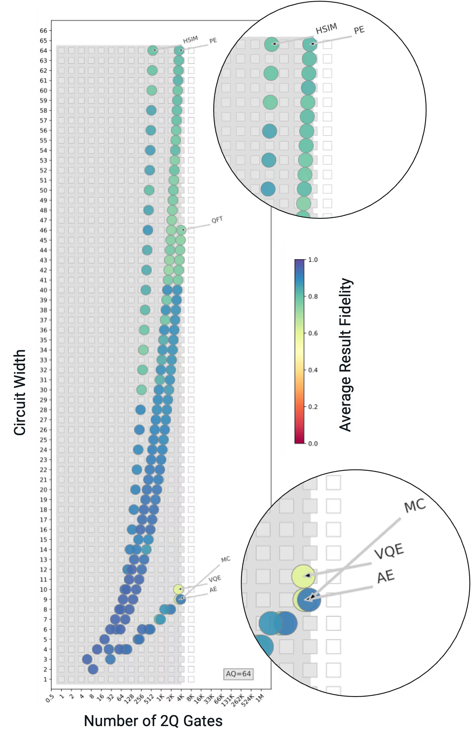
- Six instances of the most valuable quantum algorithms were run on IonQ Tempo
- #AQ Algorithms were successfully run on up to 64 qubits
- Algorithm results were deemed successful if they achieved over 37% Worst Case results fidelity
Predicting performance against your intended workloads
All of the information behind the #AQ benchmark can be summarized in a single chart that provides insight into how a system performs for a particular class of algorithms. By identifying the algorithmic classes you intend to use the system for, you can make a direct prediction about the performance of an algorithm with a specific gate width and gate depth.
Translating #AQ to real world impact
.svg)
#AQ 4
Water was simulated on IonQ Harmony, was running at #AQ 4, in 2020. The algorithm used 3 qubits across 3 parameters in the problem set and was able to produce accurate results.

#AQ 20
Lithium oxide, a chemical of interest in battery development, was simulated on IonQ Aria, running at #AQ 20, in 2022. The algorithm used 12 qubits across 72 parameters in the problem set and was able to produce accurate results.
Exponential growth: Put it into perspective
A quantum computer’s computational space, represented by the possible qubit states outlined below, doubles every time a single qubit is added to the system. Because #AQ measures a system’s useful qubits, an increase of #AQ 1 represents a doubling of that system’s computational space.
As #AQ increases, the scale becomes hard to wrap your head around. Use the below buttons to compare two #AQ metrics and explore the difference in their computational space represented by the difference in scale between two familiar objects.
Compare the scale of the computational space
Use the buttons to compare two #AQ metrics
Times smaller than

2 possible encoded states
2

4 possible encoded states
4

32 possible encoded states
32
1024 possible encoded states
1024

~66 thousand possible encoded states
66000

~8 million possible encoded states
8400000

~1 billion possible encoded states
1070000000

~69 billion possible encoded states
69000000000
~35 trillion possible encoded states
36000000000000
~2 quadrillion possible encoded states
2252000000000000
Every #AQ is built with qubits, but not all qubits result in an #AQ
A system’s qubit count reveals information about the physical structure of the system but does not indicate the quality of the system, which is the largest indicator of utility. For a qubit to contribute to an algorithmic qubit it must be able to run enough gates to successful return useful results across the 6 algorithms in the #AQ definition. This is a high bar to pass and is the reason many system’s #AQ is significantly lower than its physical qubit count.
IonQ benchmark beliefs
At IonQ, we believe benchmarks should:
Measuring algorithmic qubits (#AQ)
Define and run the algorithms
In defining the #AQ metric, we derive significant inspiration from the recent benchmarking study from the QED-C. Just like the study, we start by defining benchmarks based on instances of several currently popular quantum algorithms.
Optimization
Problems involving complex routing, sequencing and more
- Amplitude estimation
- Monte Carlo simulation
Quantum simulation
Understand the nature of the very small
- Hamiltonian
- Variational quantum eigensolver
Quantum machine learning
Problems involving complex routing, sequencing and more
- Quantum Fourier transform
- Phase estimation
Organize and aggregate the results
Building upon previous work on volumetric benchmarking, we then represent the success probability of the circuits corresponding to these algorithms as colored circles placed on a 2D plot whose axes are the 'depth' and the 'width' of the circuit corresponding to the algorithm instance.

Release updated versions of #AQ
New benchmarking suites should be released regularly, and be identified with an #AQ version number. The #AQ for a particular quantum computer should reference this version number under which the #AQ was evaluated. Ideally, new versions should lead to #AQ values that are consistent with the existing set of benchmarks and not deviate drastically, but new benchmarks will cause differences, and that is the intention - representing the changing needs of customers.

#AQ version 1.0 definition:
The success of each circuit run on the quantum computer is measured by the classical fidelity $F_c$ defined against the ideal output probability distribution:
$$F_c\left(P_{ideal}, P_{output}\right) = \left(\sum_x \sqrt{P_{output}(x) P_{ideal}(x)}\right)^2$$
where $P_{ideal}$ is the ideal output probability distribution expected from the circuit without any errors, $P_{output}$ is the measured output probability from the quantum computer, and $x$ represents each output result.
The success of each circuit run on the quantum computer is measured by the classical fidelity Fc, defined against the ideal output probability distribution:
Fc(P_ideal, P_output) = (∑ₓ P_output(x) · P_ideal(x))²
where P_ideal is the ideal output probability distribution expected from the circuit without any errors, P_output is the measured output probability distribution from the quantum computer, and x represents each possible output result.
The success of each circuit run on the quantum computer is measured by the classical fidelity $F_c$ defined against the ideal output probability distribution: $$F_c(P_{\text{ideal}}, P_{\text{output}}) = \left( \sum_x \sqrt{P_{\text{output}}(x)} P_{\text{ideal}}(x) \right)^2$$ where $P_{\text{ideal}}$ is the ideal output probability distribution expected from the circuit without any errors, $P_{\text{output}}$ is the measured output probability from the quantum computer, and $x$ represents each output result.